The Theory

Response Suface Analysis (RSA) is a method from the wider field of Response Surface Methodologies (RSM).

Requirements

1. Commensurable Scales

   Commensurability explained as briefly as possible is that two scales are measured in the same units. In the world of Likert-scales this mostly means they are measured on the same number of points.

2. Centered on a Common Point

   There is a number of ways this can be done. The most straight forward is probably to subtract scale midpoint from each participants score. This leaves participants with scores below the theoretical midpoint with negative values and everyone else with positive values.

3. Participants can indicate high and low values on all scales

   This is more of a scale design than a analysis issue. Here it is important to consider if negatively worded items should need to be included in the scale or if the lowest level of a positively worded item is the lowest score a participant could indicate.

4. No Multicolliniearity

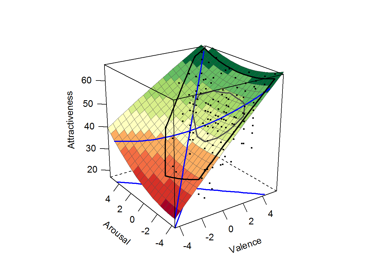
   In contrast to the previous requirement this one is actually testable. The easiest way of doing this would be to run a regression with all predictors and examine the Variance Inflation Factors (VIF). An example can be seen below where I predict attractiveness of a landscape from ratings of valence and arousal. valence and arousal are centered around the scale mid-point of 5. VIF values below 5 are generally considered acceptabily low to conclude that there is no mulitcolliniearity.

   car::vif(lm(attr ~ val_cent * aro_cent + val_cent2 + aro_cent2, data = data_long))

   ##          val_cent          aro_cent         val_cent2         aro_cent2 
   ##          4.027766          5.436807          4.003578          1.931477 
   ## val_cent:aro_cent 
   ##          4.594957

   In our current example we might have a slight multicolliniearity issue, but we are going to accept it for the purpose of the example.

5. High Power

RSA How-To

library("RSA")

## Loading required package: lavaan

## This is lavaan 0.6-3

## lavaan is BETA software! Please report any bugs.

## Loading required package: lattice

rsa_sqd <- RSA(t_attr ~ val_cent * aro_cent, data = data_long, model = "full")

## [1] "Computing polynomial model (full) ..."

summary(rsa_sqd)

## RSA output (package version 0.9.13)
## ===========================================

## Warning in sqrt(b3 * b5): NaNs produced

## Warning in sqrt(b3 * b5): NaNs produced

## Warning in sqrt(b3 * b5): NaNs produced

## Warning in sqrt(b3 * b5): NaNs produced

## Warning in sqrt(b3 * b5): NaNs produced

## Are there discrepancies in the predictors (with respect to numerical congruence)?
## ----------------------------
## Congruence
## aro_cent < val_cent          Congruence aro_cent > val_cent 
##                75.6                21.7                 2.8 
## 
## Is the full polynomial model significant?
## ----------------------------
## Test on model significance: R^2 = 0.428, p <.001
## 
## 
## Number of observations: n = 180
## ----------------------------
## 
## 
## Regression coefficients for model <full>
## ----------------------------
##                          label    est    se ci.lower ci.upper   beta
## t_attr~1                    b0 42.582 1.120   40.387   44.776  4.270
## t_attr~val_cent             b1  4.001 0.667    2.694    5.308  0.584
## t_attr~aro_cent             b2  0.914 0.540   -0.144    1.972  0.200
## t_attr~val_cent2            b3 -0.027 0.142   -0.306    0.251 -0.016
## t_attr~val_cent_aro_cent    b4 -0.180 0.156   -0.485    0.126 -0.120
## t_attr~aro_cent2            b5  0.190 0.106   -0.017    0.397  0.115
##                            pvalue sig
## t_attr~1                  p <.001 ***
## t_attr~val_cent           p <.001 ***
## t_attr~aro_cent          p = .091   †
## t_attr~val_cent2         p = .848    
## t_attr~val_cent_aro_cent p = .250    
## t_attr~aro_cent2         p = .072   †
## 
## 
## 
## Surface tests (a1 to a5) for model <full>
## ----------------------------
##   label    est    se ci.lower ci.upper   pvalue sig
## 1    a1  4.915 0.787    3.373    6.457  p <.001 ***
## 2    a2 -0.017 0.179   -0.367    0.333 p = .924    
## 3    a3  3.088 0.924    1.277    4.898  p <.001 ***
## 4    a4  0.342 0.240   -0.129    0.813 p = .154    
## 5    a5 -0.217 0.206   -0.621    0.186 p = .291    
## 
## a1: Linear additive effect on line of congruence? YES
## a2: Is there curvature on the line of congruence? NO
## a3: Is the ridge shifted away from the LOC? YES
## a4: Is there a general effect of incongruence? NO
## 
## 
## Location of stationary point for model <full>
## ----------------------------
## val_cent = 31.761; aro_cent = 12.61; predicted t_attr = 111.888
## 
## 
## Principal axes for model <full>
## ----------------------------
##                    label     est      se ci.lower ci.upper   pvalue sig
## Intercept of 1. PA   p10 100.890 189.332 -270.194  471.975 p = .594    
## Slope of 1. PA       p11  -2.779   2.382   -7.449    1.890 p = .243    
## Intercept of 2. PA   p20   1.183   2.439   -3.598    5.964 p = .628    
## Slope of 2. PA       p21   0.360   0.308   -0.245    0.964 p = .243    
##   --> Lateral shift of first PA from LOC at point (0; 0): C1 =  56.696 
##   --> Lateral shift of second PA from LOC at point (0; 0): C2 =  -0.87

# PLOT THE ESTIMATED MODEL
plot(rsa_sqd, legend=F, param=F,
     axes=c("LOC", "LOIC","PA1"), 
     project=c("LOC", "LOIC","PA1"), 
     xlab="Valence", ylab="Arousal", zlab="Attractiveness"
     )