The Background

This post is in essence a summary of McNeish’s (2018) and Raykov and Marcoulides’s (2017) “exchange” on reliability measurement using Cronbach’s alpha. I want to add a few additional perspectives to this topic and provide a short How-To in R.

What is reliability

Many students might learn what reliability is, but once they reach research praxis they often have forgotten the details and what remains is the \(\alpha > .70\) rule. To address this issue first, this rule was not suggested by Cronbach. The cut-off was suggested by Nunnally (1994). Let’s see what the original source says:

“A satisfactory level of reliability depends on how a measure is being used. In the early stages of predictive or construct validation research, time and energy can be saved using instruments that have only modest reliability, e.g., .70. If significant correlations are found, corrections for attenuation will estimate how much the correlations will increase when reliabilities of measures are increased. If these corrected values look promising, it will be worth the time and effort to increase the number of items and reduce much beyond .80 in basic research is often wasteful of time and money. Measurement error attenuates correlations very little at that level. Strenuous and unnecessary efforts at standardization in addition to increasing the number of items might be required to obtain a reliability of, say, .90. In contrast to the standards used to compare groups, a reliability of .80 may not be nearly high enough in making decisions about individuals. Group research is often concerned with the size of correlations and with mean differences among experimental treatments, for which a reliability of .80 is adequate. However, a great deal hinges on the exact test scores when decisions are made about individuals. If, for example, children with IQs below 70 are to be placed in special classes, it may make a great deal of difference whether a child has an IQ of 65 or 75 on a particular test. When selection standards are quite rigorous, decisions depend on very small score differences, and so it is difficult to accept any measurement error. We have noted that the standard error of measurement is almost one-third as large as the overall standard deviation of test scores even when the reliability is .90. If important decisions are made with respect to specific test scores, a reliability of .90 is the bare minimum, and a reliability of .95 should be considered the desirable standard. However, never switch to a less valid measure simply because it is more reliable.” (pp.264)

To boil down what Nunnally said; reliability can never replace validity, the reliability your measure should achieve is dependent on the context of application. The commonly applied rule of .70 is fitting for some contexts. Specifically contexts where one wants to save time and effort. Lance, Butts, and Michels (2006) make the important point that this is not a context that applies in most published papers. In most contexts we would want \(\alpha\) to be over .80 and over .90 | .95 if we make judgments about individuals based on this test, such as personality questionnaires used for hiring.

In the discussion on the applicability of \(\alpha\) Nunnally makes statements such as:

“Coefficient a usually provides a good estimate of reliability because sampling of content is usually the major source of measurement error for static constructs and also because it is sensitive to the”sampling" of situational factors as well as item content." (p.252)

But what is the “usual” case which Nunnally assumes. We could assume that it is the case in which the underlying assumption of \(\alpha\) are met. Let’s have a look at these assumptions to better appreciate Nunnally’s usual case. I am paraphrasing in this section from the excellent article by McNeish (2018) and I highly recommend reading it for a more detailed discussion.

1. The scale is uni-dimensional.
2. Scale items are on a continuous scale and normally distributed.
3. The scale adheres to tau equivalence.
4. The errors of the items do not covary.

Let’s step through a normal scale we could find in our data, such as well-being. Participants answered a scale on flourishing and a scale on satisfaction with life. Because we are interested in overall well-being, we decided to combine the individual items into a single score.

wll <- c("swls_1", "swls_2", "swls_3", "swls_4", "swls_5", "flourishing_1",
"flourishing_2", "flourishing_3", "flourishing_4",
"flourishing_5", "flourishing_6", "flourishing_7", "flourishing_8")

Let’s get the theoretical assumpitions out of the way first. Regarding assumption 1, we know that the scale is not uni-dimensional, because it is made up from two distinct scales. We can support this looking at the scree plot below (the paralell analysis would show one factor, but for the sake of argument let’s assume the scree is right.)

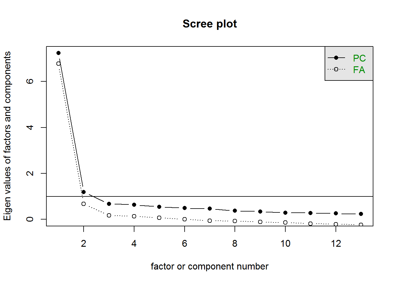
So we can see we already violate one assumption of Cronbach’s \(\alpha\). You can see similar things in many publications that first report the reliability of facets (e.g. mindfulness) and then report the overall reliability.

Assumption 2 can be split into the requirement that the data is continous, which Likert-type scales are arguably not (for disagreeing stances see: Norman 2010; Carifio and Perla 2007). For brevities sake I avoid this discussion for now, on the other hand we can assess normality of our data quite easily. As shown below none of our items is normally distributed.

##            Test      Variable Statistic   p value Normality
## 1  Shapiro-Wilk    swls_1        0.9280  <0.001      NO    
## 2  Shapiro-Wilk    swls_2        0.8924  <0.001      NO    
## 3  Shapiro-Wilk    swls_3        0.9018  <0.001      NO    
## 4  Shapiro-Wilk    swls_4        0.9118  <0.001      NO    
## 5  Shapiro-Wilk    swls_5        0.9215  <0.001      NO    
## 6  Shapiro-Wilk flourishing_1    0.9110  <0.001      NO    
## 7  Shapiro-Wilk flourishing_2    0.8474  <0.001      NO    
## 8  Shapiro-Wilk flourishing_3    0.9130  <0.001      NO    
## 9  Shapiro-Wilk flourishing_4    0.8905  <0.001      NO    
## 10 Shapiro-Wilk flourishing_5    0.8707  <0.001      NO    
## 11 Shapiro-Wilk flourishing_6    0.8644  <0.001      NO    
## 12 Shapiro-Wilk flourishing_7    0.8700  <0.001      NO    
## 13 Shapiro-Wilk flourishing_8    0.8810  <0.001      NO

Assumption 3 is also something we can test quite easily using SEM. We would just compare the fit of the unrestricted model to a model that restricts the loadings of all items on the latent variable to be identical. If we find no substantial decrease in fit we could conclude that we have tau-equivalence. There is also a number of packages that allow you to test for tau-equivalence of your data such as the coefficientalpha package (Which does not seem to be still actively developed and has not the best documentation for functions). In our current case we do not have tau-equivalence.

Assumption 4 is again something that could be easily assessed using a SEM approach. For brevities sake I will omit this, as I think my point is clear. In essence, many commonly used scales violate the assumptions of \(\alpha\). And independent of the size of the impact we should strife to use as fitting methods as possible.

Alternatives

So what are the alternatives to alpha. First I do not think that we need to replace alpha for now Raykov and Marcoulides (2017) make some interesting points on its contiued usage. So instead of replacing it, we could try supplementing it. Alternatives suggested by McNeish (2018) are omega total, and GLB. So how would we compute those reliabilities. We have a number of options from different packages, such as the psych package.

psy_omega <- psych::omega(dat[wll], nfactors = 2, poly = F)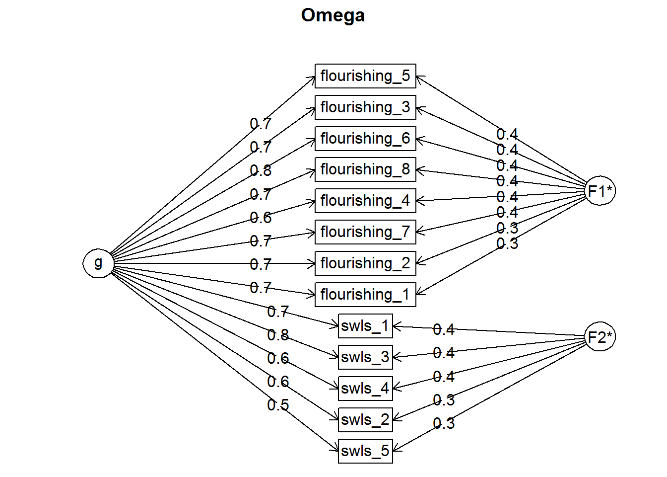

psy_omega

## Omega 
## Call: psych::omega(m = dat[wll], nfactors = 2, poly = F)
## Alpha:                 0.93 
## G.6:                   0.94 
## Omega Hierarchical:    0.81 
## Omega H asymptotic:    0.86 
## Omega Total            0.94 
## 
## Schmid Leiman Factor loadings greater than  0.2 
##                  g   F1*   F2*   h2   u2   p2
## swls_1        0.69        0.41 0.64 0.36 0.74
## swls_2        0.64        0.33 0.52 0.48 0.79
## swls_3        0.76        0.41 0.74 0.26 0.78
## swls_4        0.65        0.36 0.55 0.45 0.76
## swls_5        0.55        0.30 0.39 0.61 0.77
## flourishing_1 0.72  0.27       0.60 0.40 0.85
## flourishing_2 0.67  0.33       0.56 0.44 0.80
## flourishing_3 0.68  0.39       0.62 0.38 0.76
## flourishing_4 0.59  0.36       0.48 0.52 0.73
## flourishing_5 0.65  0.43       0.62 0.38 0.69
## flourishing_6 0.76  0.37       0.71 0.29 0.80
## flourishing_7 0.69  0.35       0.60 0.40 0.79
## flourishing_8 0.65  0.37       0.56 0.44 0.76
## 
## With eigenvalues of:
##    g  F1*  F2* 
## 5.86 1.05 0.69 
## 
## general/max  5.59   max/min =   1.51
## mean percent general =  0.77    with sd =  0.04 and cv of  0.05 
## Explained Common Variance of the general factor =  0.77 
## 
## The degrees of freedom are 53  and the fit is  0.5 
## The number of observations was  393  with Chi Square =  191.65  with prob <  1.4e-17
## The root mean square of the residuals is  0.03 
## The df corrected root mean square of the residuals is  0.04
## RMSEA index =  0.083  and the 10 % confidence intervals are  0.069 0.094
## BIC =  -124.97
## 
## Compare this with the adequacy of just a general factor and no group factors
## The degrees of freedom for just the general factor are 65  and the fit is  1.34 
## The number of observations was  393  with Chi Square =  515.94  with prob <  2.1e-71
## The root mean square of the residuals is  0.1 
## The df corrected root mean square of the residuals is  0.11 
## 
## RMSEA index =  0.134  and the 10 % confidence intervals are  0.122 0.144
## BIC =  127.65 
## 
## Measures of factor score adequacy             
##                                                  g   F1*   F2*
## Correlation of scores with factors            0.90  0.64  0.63
## Multiple R square of scores with factors      0.82  0.41  0.39
## Minimum correlation of factor score estimates 0.63 -0.19 -0.22
## 
##  Total, General and Subset omega for each subset
##                                                  g  F1*  F2*
## Omega total for total scores and subscales    0.94 0.92 0.87
## Omega general for total scores and subscales  0.81 0.72 0.66
## Omega group for total scores and subscales    0.12 0.20 0.20

I personally prefer the userfriendlyscience package, which containts the niffty reliability function.

sci_omega <- userfriendlyscience::reliability(dat[wll])

## 
## Information about this analysis:
## 
##                  Dataframe: data
##                      Items: swls_1, swls_2, swls_3, swls_4, swls_5, flourishing_1, flourishing_2, flourishing_3, flourishing_4, flourishing_5, flourishing_6, flourishing_7, flourishing_8
##               Observations: 393
##      Positive correlations: 78 out of 78 (100%)
## 
## Estimates assuming interval level:
## 
##              Omega (total): 0.93
##       Omega (hierarchical): 0.81
##    Revelle's omega (total): 0.95
## Greatest Lower Bound (GLB): 0.96
##              Coefficient H: 0.94
##           Cronbach's alpha: 0.93
## Confidence intervals:
##              Omega (total): [0.92, 0.94]
##           Cronbach's alpha: [0.92, 0.94]
## 
## Estimates assuming ordinal level:
## 
##      Ordinal Omega (total): 0.94
##  Ordinal Omega (hierarch.): 0.93
##   Ordinal Cronbach's alpha: 0.94
## Confidence intervals:
##      Ordinal Omega (total): [0.93, 0.95]
##   Ordinal Cronbach's alpha: [0.93, 0.94]
## 
## Note: the normal point estimate and confidence interval for omega are based on the procedure suggested by Dunn, Baguley & Brunsden (2013) using the MBESS function ci.reliability, whereas the psych package point estimate was suggested in Revelle & Zinbarg (2008). See the help ('?scaleStructure') for more information.

#References