#MDS basics
This post focuses on MDS (Also sometimes called smallest space analysis (Guttman, 1968) or multidimensional similarity structure analysis (Borg & Lingoes, 1987)) as exploratory tool and a large amount of the information is lifted from Borg and Gronen (2005) which I really recommend for further readings.
Exploratory MDS might seem at first glance like tea-leaf reading, but over the years several rules have been developed that aid in determining structure from the MDS plots.
In the case I will talk about during this post we were interested in discovering how different measures of mindfulness, personality, and approach/ avoidance motivation are related to each other. To this extent participants answered statements about themselves on Likert-scales related to these concepts. An important concept in MDS is distance. The idea behind distance is that individuals reproduce mental distances between concepts when asked about dissimilarities between the concepts. To cite directly form Borg and Gronen (2005):
“The most common approach is to hypothesize that a person, when asked about the dissimilarity of pairs of objects from a set of objects, acts as if he or she computes a distance in his or her “psychological space” of these objects."
In our case participants were not asked to rate dissimilarities between the measures, but rather rate themselves on these measures. Nevertheless, if we think about it these self-ratings can also represent psychological distances. A participant that scores high on avoidance behaviour might also score high on anxiety, but score low on approach behaviour. These differences can be represented as psychological distances with avoidance behaviour and anxiety being in close proximity and approach behaviour being distal from those two concepts. ## Comparing MDS and PCA
Mathematically and conceptually, there are large similarities between MDS and Principal components analysis (PCA) or factor analysis. PCA is more focused on the dimensions themselves, and seek to maximize explained variance, whereas MDS is more focused on relations among the scaled objects.
Correlations and MDS
Data obtained from answers to Likert scales can not directly be considered as distances, but the correlation coefficients between multiple columns can. Correlations are appropriate for MDS.
Obtaining a distance matrix from a correlation matrix.
The psych package provides a handy function (cor2dist) to transform a correlation matrix into a distance matrix. In the background this simple function is performed: \[\sqrt{2 * (1 - x)}\]
Pipelines provide a handy way of reducing the number of objects stored in the work space if they are not used in later analysis. In my current case I used the different measures of interested (Mindfulness facets, personality, etc.) and labeled the facets. The first line produces the correlation between the variables, the second line selects only the correlation coefficients from the output, and the second line converts them into a distance matrix which is returned as an object labelled distance.
distance <- psych::corr.test(mnd_test[,facets]) %>%
  .$r %>%
  psych::cor2dist()
So why even bother with transforming correlation coefficients into distances? The reason for this can be found in the assumptions about a geometrical plane. The first assumption is called non-negativity and can be expressed as: \[d_{ii} = d_{jj} = 0 ≤ d_{ij}\] Simply put on plane the the distance between any two points \(i\) and \(j\) is greater than 0 or equal to 0 (if \(i = j\)). This presents the first reason why correlation coefficients can not directly used as input for a MDS, because they can be negative. The second assumption called symmetry is self-explanatory: \[d_{ij} = d_{ji}\] For an MDS it is necessary that the distance between \(i\) and \(j\) is identical to the distance between \(j\) and \(i\).
Last is the triangle inequality: \[d_{ij} ≤ d_{ik} + d_{kj}\]
This triangle inequality says that going directly from \(i\) to \(j\) will never be farther than going from \(i\) to \(j\) via an intermediate point \(k\). If \(k\) happens to be on the way, then the function is an equality.
Evaluating stress
Rather then goodness-of-fit indicators MDS uses a badness-of-fit indicator, stress. Stress is the normed sum of squares aggregating the representation errors of the model compared to the underlying data. In an applied context we rarely examine the raw stress scores as it is dependent on the scale used. Rather we use a value to judge badness-of-fit that is called Stress-1 or \(\sigma_1\) 1 (Kruskal, 1964a). If you are interested, below is the formula for \(\sigma_1\).
\[\sigma_1(X) = \sqrt{\frac{\sum{[f(p_{ij}) - d_{ij}(X)]^2}}{\sum{d_{ij}^{2}(X)}}}\]
One important property of \(\sigma_1\) is that missing data is skipped in the process of summing up the representation errors. The more missing data is present the lower the stress value will be. This is probably less a problem if you are working with correlations derived from underlying data, but can be a problem if you are working with values obtained from other sources.
From the presented formula we can derive that if we perfectly represent the underlying data \(\sigma_1\) will be 0 and the greater the deviation gets the greater \(\sigma_1\) becomes.
Determening the correct number of dimensions
All data can be represented in a MDS with 0 stress in \(m = n -2\) dimensions, where \(m\) is the number of dimensions and \(n\) is the number of variables included in the MDS. Borg and Gronen again express this dilemma in a very succinct way :
“However, such perfect solutions are not desired, as we saw above. Therefore, one seeks an MDS representation with considerably fewer dimensions. The problem is how to choose the “proper” dimensionality. Scaling with too few dimensions may distort the true (reliable) MDS structure due to over-compression or may lead to technical problems. Being too generous on dimensions may, on the other hand, blur the MDS structure due to overfitting noise components."
As everything in MDS the decision on the number of dimensions is largely up to the researcher and while universal rules of thumb are hard to give several methods have been developed to assists applied researchers to determine the correct number of dimensions.
One method should be familiar to anyone that uses factor analysis on the regular, the scree plot (Or parallel analysis). The goal is to fin a solution “for which further increase in [m] does not significantly reduce Stress” (Kruskal, 1964a, p. 16). The simplest way to do this is computing the \(\sigma_1\) for each m-dimensional solution and plotting it against the number of dimensions. This can easily be done in R using many different approaches, below is a very lazy implementation with a for loop.
## The for loop runs the MDS function for the amount of variables in the set - 1.
for(ii in 1:(length(facets) - 1)){
            distance_MDS <- smacof::mds(distance, ndim = ii,
                                        type =   "ordinal")
            randomstress <- smacof::randomstress(37, ndim = ii, nrep = 10,
                                                 type = "ordinal")
            randomstress_value[ii] <- mean(randomstress)
            stress_values[ii] <- distance_MDS$stress
}
## Registered S3 methods overwritten by 'car':
## method from
## influence.merMod lme4
## cooks.distance.influence.merMod lme4
## dfbeta.influence.merMod lme4
## dfbetas.influence.merMod lme4## Here I just add a second column that contains the number of dimension corresponding to the stress value.
stress_plot <- cbind(stress = stress_values,
dimension = seq(1:(length(facets) - 1)),
random_stress = randomstress_value) %>%
as.data.frame() %>%
gather(., key = "type", value = "stress", -"dimension")
stress_plot$diff <- ave(stress_plot$stress, stress_plot$type,
FUN = function(x) c(0, abs(diff(x))))
## Last, I plot the number of dimensions on the x-axis and the stress-1 value on the y axis.
stress_plot %>%
ggplot() +
aes(x = dimension, y = stress, colour = type) +
geom_point() +
geom_line() +
theme_classic()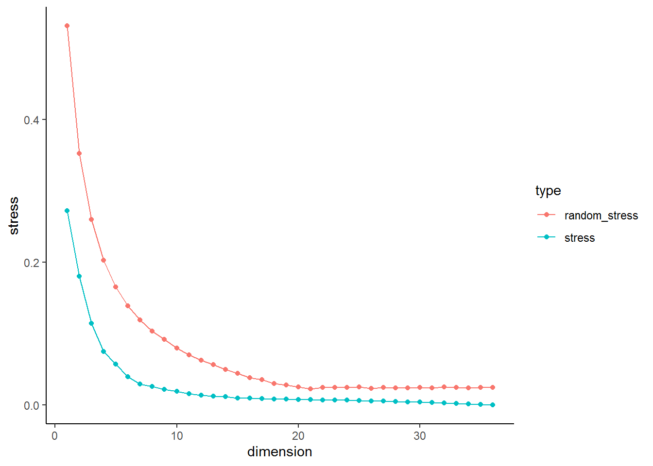
This plot can be inspected to determine the appropriate number of dimensions. As you can see stress is monotonically decreasing with increasing dimensionality. At the start a step decline occurs and after a certain point stress decreases only marginally with increasing dimensionality. A commonly applied interpretation is to look for the elbow of the scree plot, where decreases in stress become less pronounced. The rationale of this choice is that the elbow marks the point where MDS uses additional dimensions to essentially only scale the noise in the data, after having succeeded in representing the systematic structure in the given dimensionality m.
I find it also quite useful to look at the distance in stress between \(n\) and \(n + 1\). The plot below plots the difference in stress for each dimension in respect to the previous dimension (It is obviously 0 for the first dimension, therefore the plot starts with \(n = 2\)). We can see that the difference between \(n = 1\) and \(n = 2\) is similar in real and simulated data. The pattern remains the same in real and simulated data until \(n= 5\) and \(n = 6\). At this point we see a clear deviation in the real data from the pattern in the random data. This could indicate that this could be considered the point of inflection.
stress_plot %>%
ggplot() +
aes(x = dimension, y = diff, colour = type, group = type) +
geom_point() +
geom_step() +
xlim(2, max(stress_plot$dimension)) +
theme_classic()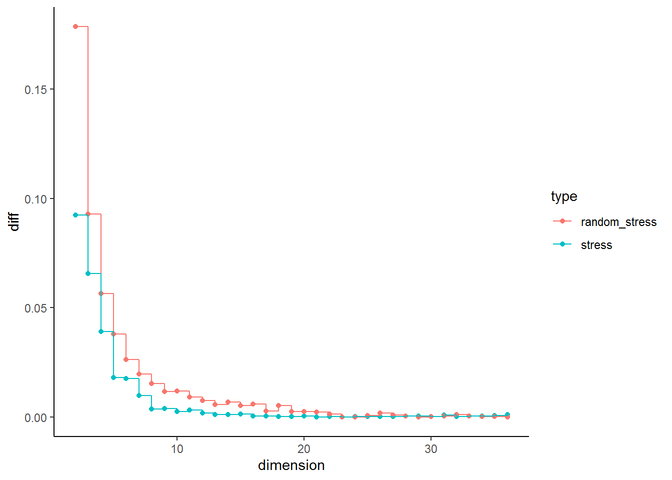 I mentioned parallel analysis above. Some simulation studies on stress obtained from random data based on different n and m were conducted in the past (Cliff, 1973; Knoll, 1969; Klahr, 1969; Spence and Ogilvie, 1973). It might be promising to implent an approach that mirrors parallel analysis for stress values.
In our current example this point could be point 4 based on the stress plot or 5/6 based on looking at drop in stress. A further problem that needs to be considered in MDS that if one intends to plot the resulting graph dimensions above 3 are hard to display and visually interpret. This makes trade offs between the goal of MDS, uncovering and visualising data structures, and statistical rigor necessary. I would use 3 dimensions, as they can still be visualised and their \(\sigma_1\) = 0.11 is low enough to assume acceptable representation of the underlying data.
So what is a acceptable stress value? Often quoted or rather misquoted at this point is Guttman (in Porrat, 1974). If you have a look online and even in some publications authors report that \(\sigma_1 <= .15\) represents a good value for an acceptably precise ordinal MDS solution. Citing again from Borg and Gronen:
“[H]e required that the coefficient of alienation K [which is similar but not identical to Stress] should be less than 0.15 for an acceptably precise MDS solution. He later added that what he had in mind when he made this proposal were “the usual circumstances”(Guttman, personal communication)."
The usual circumstances are where the number of items clearly exceeds the number of dimensions (sometimes suggested as \(n > m * 4\)). Further if \(n > m * 10\) larger values than .15 are acceptable. I did a small literature search, but could not find any studies that directly compared the coefficient of alienation K to \(\sigma_1\). In my view it is unclear how well the .15 rule translates between those measures.
Other authors developed recommendations based on experience for \(\sigma_1\). The following part from Borg and Gronen highlight an exceptionally important point about those cut-offs:
“For the Stress-1 coefficient σ1 using ordinal MDS, Kruskal (1964a), on the basis of his “experience with experimental and synthetic data” (p. 16), suggests the following benchmarks: .20 = poor, .10 = fair, .05 = good, .025 = excellent, and .00 = perfect. Unfortunately, such criteria almost inevitably lead to misuse by suggesting that only solutions whose Stress is less than .20 are acceptable, or that all solutions with a Stress of less than .05 are good in more than just a formal sense. Neither conclusion is correct. An MDS solution may have high Stress simply as a consequence of high error in the data, and finding a precise representation for the data does not imply anything about its scientific value. "
We can see in the stress plot that we could further reduce \(\sigma_1\) and increase the granularity of our analysis if we increase the number of dimensions. On the other hand we might sacrifice interpretability of the final solution. If you are interested in the analysis with a greater number of dimensions, feel free to use the underlying data.
##Plotting the solution
MDS <- smacof::mds(distance, type = "ordinal", ndim = 3)
coordinates <- as.data.frame(MDS$conf) %>%
  tibble::rownames_to_column()
library(plotly)
p <- plot_ly(coordinates,
                     x = ~D1,
                     y = ~D2,
                     z = ~D3) %>%
  add_markers(name = ~rowname,
              opacity = .80)

p
Interpretation of a MDS plot
In their introduction to Multidimensional Scaling Kruskal and Wish recommend that a MDS plot should be interpreted by applying the following rule (generalised from their example of Morse code): " Pick some point which is peripheral, that is, which lies at the outermost edge of the configuration. Ask yourself what is common to this point and its nearest neighbors, and how they differ from the points at the opposite edge of the configuration. Then repeat this process, using other peripheral points."
In a two dimensional plot it can be beneficial to first examine the x and y axis. This can yield important insight into the structure of the points. Same holds true for a 3-dimensional solution. We first look at x, y, and z.