This is a very short post in which I want to highlight, because I realized that the issue is often overlooked by students when writing up their data. Today I want to highlight the difference between within- and between-subjects errors (With code examples).
Imagine you have data like this example below. Participants responded to a number of mindfulness items multiple times during the day over the duration of a week. For simplicity, I will only focus on days and not events during the day.
## # A tibble: 6 x 8
##   number   day sms_1 sms_2 sms_3 sms_4 sms_5 sms_6
##    <dbl> <dbl> <dbl> <dbl> <dbl> <dbl> <dbl> <dbl>
## 1  18072     1     8     9     8     8     8     8
## 2  18072     1     8     8     8     8     9     8
## 3  18072     1     8     8     6     9     9     9
## 4  18072     1     6     7     6     8     9     9
## 5  18072     3     7     7     7     8     8     8
## 6  18072     3     8     8     8     8     8     8
A natural first instinct if you have similar data would be to compute the means and standard errors, which would be fine if each row would be an independent observation. In our case this is not the case each participant answered seven surveys and the distinct possibility exists that some of the variance might be due to difference between participants. In R there is an easy way to account for this (if you want to read more on the theoretical background I recommend Morey 2008; Franz and Loftus 2012; Cousineau 2017).
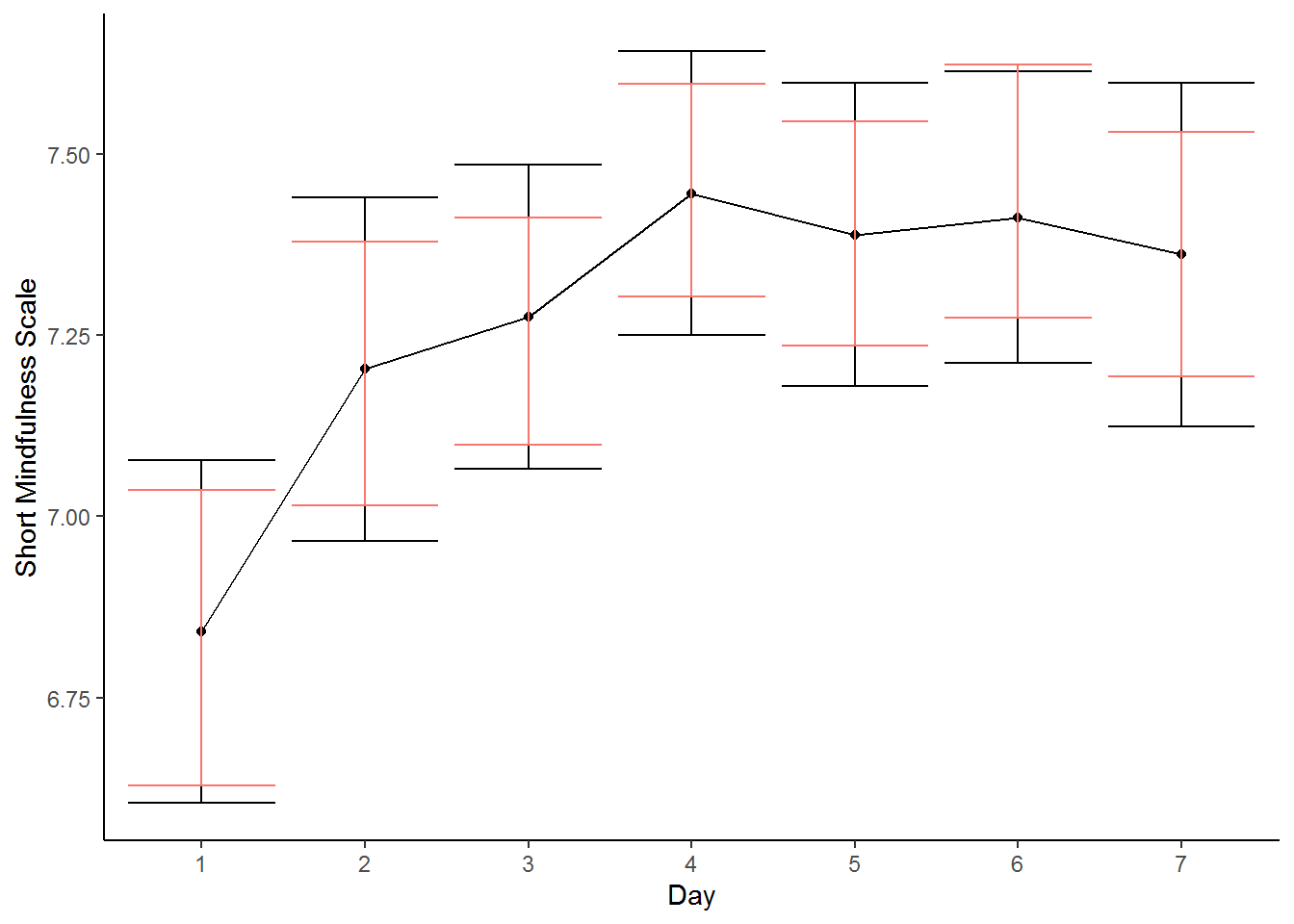
The first function (Rmisc::summarySE) computes errors without considering that the observations are not independent. The second function (Rmisc::summarySEwithin) computes the errors accounting for the non-independent nature of the observations. We can now see that after only three days of journaling participants report higher scores of mindfulness, whereas using between-subjects errors we would conclude that there is no difference between the values on the third day and the baseline.
between <- Rmisc::summarySE(data = data_long, measurevar = "sms",
                            groupvars = "day")

within <- Rmisc::summarySEwithin(data = data_long, measurevar = "sms",
                                 withinvars = "day",
                                 idvar = "number")

within$day <- as.integer(within$day)
Plotting the two different solutions, we can clearly see the difference. The between-subjects errors are in black and the within-subjects errors are in red. The within-subjects errors are considerably smaller as a result of accounting for the non-independence.
ggplot(between, aes(x = factor(day), y = sms, group = 1)) +
  geom_line(stat = "identity") +
  geom_point() +
  geom_errorbar(aes(ymin = sms - ci, ymax = sms + ci)) +
  geom_errorbar(aes(ymin = sms - ci, ymax = sms + ci,
                    colour = "red1"), data = within) +
  guides(colour = FALSE) +
  labs(x = "Day", y = "Short Mindfulness Scale") +
  theme_classic()
Cousineau, Denis. 2017. “Varieties of Confidence Intervals.” Advances in Cognitive Psychology 13 (2). University of Finance; Management in Warsaw: 140–55. https://doi.org/10.5709/acp-0214-z.
Franz, Volker H, and Geoffrey R Loftus. 2012. “Standard errors and confidence intervals in within-subjects designs: generalizing Loftus and Masson (1994) and avoiding the biases of alternative accounts.” Psychonomic Bulletin & Review 19 (3). Springer: 395–404. https://doi.org/10.3758/s13423-012-0230-1.
Morey, Richard D. 2008. “Confidence Intervals from Normalized Data: A correction to Cousineau (2005).” Tutorials in Quantitative Methods for Psychology 4 (2): 61–64. https://doi.org/10.20982/tqmp.04.2.p061.
